Study on the spatial – temporal distribution of atmospheric water content with the combined use of satellite remote sensing and non-linear science  
EN GR


Project Description

Methodology

PW Derivation Methodology
Theoretical analysis proposes an almost linear relationship between PW and ΔT, with slope and intercept being determined by the surface emissivity. As is has been shown in past studies the PW is proportional to the difference between the two AVHRR thermal channels brightness temperature.

This split-window technique is not a universal solution to PW retrieval due to the dependence of the difference ΔT on air temperature and surface characteristics. Linear relationships characterized by different coefficients are expected to hold in different locations. The coefficients of the linear relationship between PW and ΔT are site specific.

In this study, MODIS derived PW were used as an independent dataset, adjusted for the time lag between the time of Terra/MODIS and NOAA16/AVHRR overpasses. Radiosonde data were used for this adjustment. More specifically, if the AVHRR acquisition over the study area is performed at t = t0, the PW at this time, PW(t0), can be estimated as linear function of ΔΤ:

where, a and b are coefficients that need to be estimated for the study area, and ΔΤ = T4 – T5 is the brightness temperatures for channels 4 and 5 in the (x, y) cell.
By a Taylor's series expansion of PW about the time t0 we obtain:

where,

Δt = t - t0 is the time difference between MODIS and AVHRR passes,
  is the partial derivative of PW with respect to time, being evaluated at  t=t0. It represents the rate of change of PW.

Therefore, the MODIS derived PW can be related to the AVHRR derived ΔT as:

The term  represents an estimation of the actual precipitable water during the AVHRR acquisition time called the adjusted precipitable water (PW*).  PW* was computed by combining MODIS derived PW with radiosonde derived PW rates of change over the study area. The latter was derived by spatial interpolation using the PW rates of change calculated at the synoptic stations of Athens, Thessaloniki, Heraklion and Izmir. Consequently, the Equation (3) can be written as:

The coefficients a and b in (4) were estimated by linear regressions of PW* vs ΔΤ. In this study, the estimation of the coefficients a and b was based on MODIS, AVHRR and radiosonde data acquired during 15 selected days of 2003 and 2004.

The selection criteria for these days were: a) As much cloud free land area as possible and b) near nadir NOAA16/AVHRR acquisitions over the study area. The aerosol concentration was low, since meteorological horizontal visibilities greater than 10 km are observed in all cases. Moreover, the values of horizontal visibilities, suggested that there was no Saharan dust episode, thus it was assumed that the aerosol haze had a small effect in observed radiances.

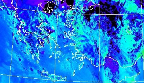
The estimated PW* – ΔΤ relationship was applied to AVHRR data to provide PW spatial distributions for the period 2001 – 2005 (for January, April, July and October).


PW Non-Linear Analysis Methodology
Nonlinear time series analysis is a powerful tool to explore complex phenomena. In this project satellite remote sensing combined with nonlinear physics was used. More specifically the powerful nonlinear cross-prediction error approach in combination with wavelet packet decomposition was used to perform nonlinear time series analysis for rainstors. Some areas in Greece, in the middle and lower reaches of Yangtze River and in the Huaihe River basin in China were selected for this study. The data that were used consist of satellite derived values of precipitable water values (PW), brightness temperature Tb, and land surface temperature Tg. and conventional observations derived values of atmospheric temperature and water vapor at some atmospheric levels and on surface, which were available mainly from global assimilation data of NOAA/NCEP(National Centers for Environmentl Prediction). Due to lack of some values, three methods of data interpolations were performed. (cubic spline, fractal and neural network interpolations) The non linear calculations separated in the four following steps:

  1. Check if the rainstorm process time series are stationary
  2. Reconstruction of the phase space with the embedding dimension m for the time series  
  3. Fractal correlation dimension, Lyapunov exponent spectrum, and the largest Lyapunov exponent
  4. Finally, using nonlinear cross prediction error approach combined with wavelet packet decomposition to perform calculations for different frequency levels of nonlinear time series for the multi-source observation data.
It should be pointed out that the correlation dimensions for the time series with rainstorm processes investigated are 3.0 ~ 4.0, and the largest Lyapunov exponent values are mainly in 0.05 ~ 0.20. These results are incorrect mainly due to the not enough time series data in the time series. Furthermore, the calculation results show that the time series investigated is non-stationary, which means that the rainstorm processes do not belong to chaos motion, but have more complex and nonlinear behavior. So, we turn to use more powerful nonlinear cross prediction error approach with wavelet packet decomposition to study the subject. Analyzing the curves of nonlinear cross-prediction error vs time for the cases of rainstorm processes, we find that a characteristic curves peak appears around 5-15 days ahead of the rainstorm processes. The result indicates that it is promising to combine satellite remote sensing and other conventional observations with nonlinear physics approach to set up a novel model for monitoring and prediction of rainstorm processes. However, more cases of nonlinear time series containing rainstorm processes need to be studied to further verify the results.